 On first day at work, I was given an excel workbook that was used to test the reports which are generated using a software and are delivered to the client. The workbook had a large amount of data, kind of a database in itself and we had to use this huge data set and bring the data into a format that is conceivable to us so that reports that are prepared can be tested. It had used Pivot Table to summarize the data. I came across the concept of pivot table when I was formally taught elementary excel in eighth grade, the learning was more theoretical than practical, I did make few pivot tables here and there but it wasn’t the Swiss knife in my toolkit like now.
In this post I am going to introduce you to the concept of the pivot tables and create one for a little hands-on exercise. Today, I use pivot tables on a daily basis and it has become a second nature of mine. By the end of this series I hope you will too find Pivot table as a Swiss Knife in your toolkit and not an Achilles heel. This is the first in the series of the tutorial dealing with Pivot tables. But before we jump into it let us get some theoretical insight into the Pivot Tables.
Pivot table, as mentioned above is a data summarization tool. A pivot table is an interactive worksheet table that quickly summarizes large amounts of data using calculation methods you choose. It is called a pivot table because you can rotate its row and column headings around the core data area to give you different views of the source data.
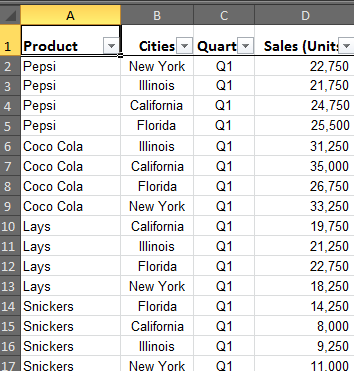
Download the workbook for practice here. I am presenting the sales of products in various states in different quarters as an example. I want a simple report which consolidates the Sales for a particular product in different states in a particular quarter. Let us try this without using the Pivot table. (Using MS-Excel 2007/2010)
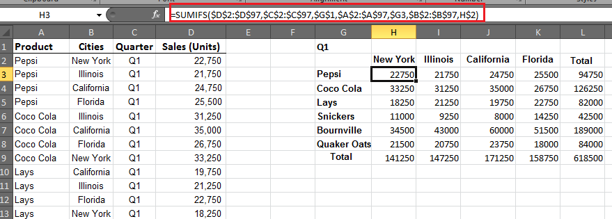
So I re-enter the various unique states in a row as a header and name of the products as a column the intersection will of course present the consolidated sales of a product in a state during a particular quarter, which is mentioned in a cell above the header row. The screenshot shows how this can be achieved.
As you must have understood we need to use SUMIFS function for this purpose to impose the three on the sum that is to be calculated on the sales. For the earlier version of excel, prior to MS-Excel 2007,
the SUMIFS function is not present so an even more complicated formula needs to be used in its place to carry out the desired summation. The formula used to for the first cell in the grid is as follows and extending the formula to the other cells will populate the grid fully.
=SUMIFS($D$2:$D$97,$C$2:$C$97,$G$1,$A$2:$A$97,$G3,$B$2:$B$97,H$2)
The Total Column contains the usual Sum of the sales at product level across the states (present on the right hand side of the table) and Total Row contains the Sum of Sales at State level (present at the bottom of the table). The formula is not very tough and is at back of the hand for many excel users but if the data summarization operation became tougher the formulae will be more in number and higher in complexity
This entire process can be achieved by few mouse clicks and drag and drops. Let’s do this now.
1.Select the entire data set including the headers and select Insert from the ribbon and click on Pivot Table.
2.This will prompt the following window where the range of the selected data is present and we can give the location where we want the pivot table to be. You can either insert this in a new worksheet or you can place it in the current sheet by specifying the cell range of the destination.

3.Now you can see the Pivot table Field List Window on the right side of the Excel window. If you don’t see it then click the Pivot table area that is appearing in the selected location in Step2 and click on the PivotTable Tools appearing over the ribbon and click on Field List in the Show section. The List is self-explanatory and is the first step toward building your Pivot table.
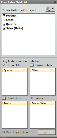
4.Take a look at the various sections of the Pivot table Field List Window. By placing the appropriate fields in appropriate section the desired Pivot Table can be obtained.

5.As per the screen shot above place the required fields in appropriate section of the Field List to get a Pivot table Field List similar to the following.
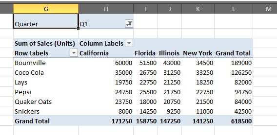
6.The Pivot Table now contains data that is summarized for all the Quarters. But as per the requirement data for just one Quarter (Q1) is required. Now Select the Report Filter for this purpose as shown below.

7.The Final Pivot is obtained as shown below, note that it is same as the one we created using the Formulae.
So this is how we create a simple Pivot Table, you can do a lot more with this as you’ll see in the coming tutorials in the series. But please try things out by yourself explore the Pivot Table Options and try getting a grasp of things. That’s all from my side for now. In the next tutorial we are going to add a few functions to the Pivot tables and make it more dynamic.
Cheers!
